In this version
- New microcontroller
- Novel LED pulsing
- Advanced speed of sound algorithm
New microcontroller
The first hardware change involved debugging button debouncing, a condition whereby a single button press gets registered multiple times. The source of this problem is the change in voltage-level rebounding amongst the components in the circuit thereby creating a noisy signal before finally settling on a high or low state. To solve the problem I created a low-pass filter using a capacitor, two resistors, and an inverting Schmitt trigger. The correct capacitor and resistor values were calculated based on the specifications of my Schmitt trigger and using the equation below.

While the same effect could be achieved using software, hardware button debouncing is relatively inexpensive, requiring only four additional low-cost components. It also reduces the amount of code run by the button interrupt function. In my opinion, hardware button debouncing is a (much) cleaner solution to the problem.
Second, I changed the operating voltage of the analog temperature sensor from 5V to 3.3V because it yields a more accurate reading. I also added another low-pass filter across the temperature sensor using a ceramic capacitor to reduce noise and create a more stable reading (and thus a more stable distance computation).
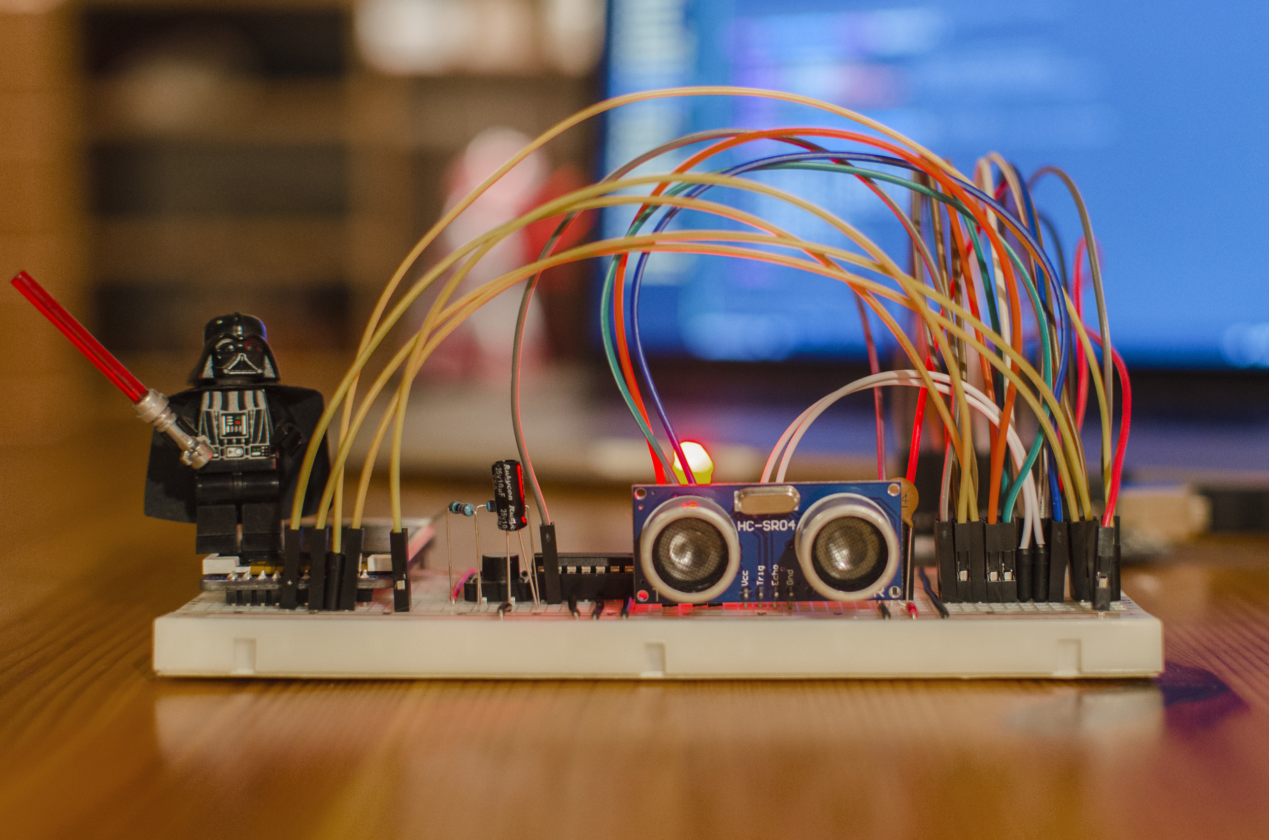
Most significantly, I changed Quantus' microcontroller from an Intel Edison to an ATMEGA328P. The original Quantus prototypes used an Intel Edison processor which boasts a 22nm Silvermont dual-core Intel Atom CPU with cores clocked at 500MHz and 100MHz, 4GB of Flash memory, and 1GB of RAM. At ~$80 it is also very expensive. Ultimately, I wanted to use an ATMEGA328P microcontroller (used by the Arduino UNO) which is inexpensive by comparison while still containing all the necessary I/O ports. However, the ATMEGA328P contains a slow 16MHz processor, 32KB of Flash memory, and only 2KB of RAM. To make the switch from the Intel Edison to the ATMEGA328P, I needed to optimize the code so it could still collect data at 20Hz. Two software optimizations towards this goal are described below.
Novel LED pulse
Quantus uses an RGB LED to communicate with the user. I wanted to add some life to Quantus by pulsing the LED because showing a single, static colour can be associated with the device being "unresponsive". I implemented timer interrupts to clean up the code and ensure that the LED pulses are timed accurately. Given that interrupts pause the internal timer, I disable the LED pulsing when collecting data and instead use a solid green colour. The LED blinks white each time a measurement is taken so that Quantus never feels unresponsive.
My first instinct was to fade linearly between two colour shades because this is easy to do and does not require much computation. However, the linear pulsing seemed very unnatural and mechanical. My next idea was to use a sinusoidal pulse following the equation below to pulse the LED.

However, this equation still seemed seemed too mechanical. I want the LED to "breathe". The following equation seemed to do the trick. I call it the respiration equation.

A graphic comparison of the two equations is below.
However, the respiration equation takes time to compute and has the potential to slow down Quantus, especially when performing tasks such as reading and writing to an SD card. My first idea to speed up the pulse computation was to store each value of the function from 0 to 2π in an array in steps of 128x/π. This method allowed me to have a very smooth LED pulse. However, storing an array of 256 unsigned 8-bit integers caused program memory issues since I only have 2KB to run Quantus' entire program. Next, I tried halving the array size so the array contains steps of 256x/π. While this fixed the memory issued, it caused the LED to stutter and not have the seamless pulse I was after. Array sizes that were smaller by factors of 2/3, 3/4, and even 5/6 still caused the LED to stutter. Therefore, I needed to develop a new method to pulse the LED in a natural way without running into memory issues.
After noticing that the function is symmetrical from 0 to π and π to 2π, I created two separate arrays, Array A and Array B, containing the respiration equation values in steps of 128x/π from 0 to π/2 and π to 3π/2, respectively. I then wrote a function to traverse Array A forwards from 0 to π/2, Array A backwards form π/2 to π, Array B forwards from π to 3π/2, and Array B backwards from 3π/2 to 2π. The only computation I need to do involves simple addition/subtraction to traverse the array in the correct direction. I can still have a small step difference 128x/π and a seamless respiration pulse while using only half the memory (compared to the original method)!
Although this may seem like a lot of dedication for only a minor difference, to me the end result was worth it, and I had fun and learned a lot implementing it.
New speed of sound algorithm
The new speed of sound algorithm is based on Owen Cramer's research (citation below) computing the speed of sound in air based on the ambient temperature, pressure, humidity, and carbon dioxide concentration.
J. Acoust. Soc. Am. 93, 2510 (1993); http://dx.doi.org/10.1121/1.405827
Originally, I computed the speed of sound in air every time I collected a data point. However, the temperature does not change significantly (or at all) between measurements. Using a linear approximation provides a reasonably accurate speed of sound value while requiring much less arithmetic.
To do the linear approximation (equation below), I take an initial temperature measurement and compute the speed of sound in air using the full algorithm. I then compute its derivative. All subsequent calculations use the linear approximation based on the originally competed value.

Additionally, I used fixed-point arithmetic (instead of double floating point arithmetic) to perform the calculations when collecting data.
The combination of the linear approximation and fixed-point arithmetic optimizations decreased the time required to collect data by 18.5%. This efficiency is required to collect data at 20Hz.